拡散確率モデル : (1) スコアマッチング (翻訳/解説)

翻訳 : (株)クラスキャットセールスインフォメーション
作成日時 : 09/15/2022 (No releases published)

* 本ページは、Denoising diffusion probabilistic models の以下のドキュメントを翻訳した上で適宜、補足説明したものです：

README.md
Diffusion probabilistic models – Score matching (Author : Philippe Esling (esling@ircam.fr))

* サンプルコードの動作確認はしておりますが、必要な場合には適宜、追加改変しています。
* ご自由にリンクを張って頂いてかまいませんが、sales-info@classcat.com までご一報いただけると嬉しいです。

クラスキャット人工知能研究開発支援サービス

◆ クラスキャットは人工知能・テレワークに関する各種サービスを提供しています。お気軽にご相談ください :

人工知能研究開発支援
1. 人工知能研修サービス(経営者層向けオンサイト研修)
2. テクニカルコンサルティングサービス
3. 実証実験(プロトタイプ構築)
4. アプリケーションへの実装
人工知能研修サービス
PoC(概念実証)を失敗させないための支援

◆ 人工知能とビジネスをテーマに WEB セミナーを定期的に開催しています。スケジュール。

お住まいの地域に関係なく Web ブラウザからご参加頂けます。事前登録 が必要ですのでご注意ください。

◆ お問合せ : 本件に関するお問い合わせ先は下記までお願いいたします。

株式会社クラスキャット セールス・マーケティング本部セールス・インフォメーション
sales-info@classcat.com ; Web: www.classcat.com ; ClassCatJP

拡散確率モデル (1) スコアマッチング

このノートブックは拡散確率モデルに基づく新しいクラスの生成モデルを調べます [1]。このクラスのモデルは熱力学からの考察にインスパイアされていますが [2]、ノイズ除去スコアマッチング [3]、ランジュバン動力学と自己回帰デコーディングへの強い類似性もまた持っています。ノイズ除去拡散暗黙モデル [4] のより最近の開発についても考察します、これはサンプリングを高速化するためにマルコフ連鎖の必要性を迂回します。このワークに由来し、wavegrad モデル [5] についても考察します、これは同じコア原理に基づきますが、音声データのためにこのクラスのモデルを適用しています。

拡散モデルの内部動作を完全に理解するため、関連トピックの総てをレビューします。そのため、説明を 4 つの詳細なノートブックに分割します。

スコアマッチングとランジュバン動力学。
拡散確率モデルとノイズ除去
WaveGrad による waveforms への応用。
推論を高速化するための暗黙モデル

スコアマッチング

このセクションではスコアマッチングの基礎の総てをレビューすることから始めます、これは拡散モデルを完全に理解することにつながります。そのため、伝統的なスイスロール・データセットに取り組みます。

%matplotlib inline
import matplotlib.pyplot as plt
import numpy as np
from sklearn.datasets import make_swiss_roll
from helper_plot import hdr_plot_style
hdr_plot_style()
# Sample a batch from the swiss roll
def sample_batch(size, noise=1.0):
    x, _= make_swiss_roll(size, noise=noise)
    return x[:, [0, 2]] / 10.0
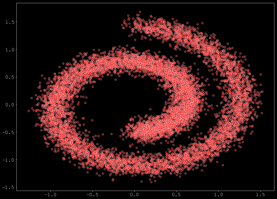
# Plot it
data = sample_batch(10**4).T
plt.figure(figsize=(16, 12))
plt.scatter(*data, alpha=0.5, color='red', edgecolor='white', s=40)

スコアマッチングのアイデアは元々は Hyvarinen et al. [6] により提案されました。データの確率 $\log p(\mathbf{x})$ を直接学習する代わりに、$x$ に関する $\log p(\mathbf{x})$ の勾配を学習することを目標とします。この場合、勾配 $\nabla_{\mathbf{x}} \log p(\mathbf{x})$ は密度 $p(\mathbf{x})$ のスコアと呼称され、従って名前はスコアマッチングになります。これは入力空間の各ポイントにおける最も確率の高い方向を学習するものとして理解できます。従って、モデルが訓練されるとき、それを最も高い確率の方向に沿って移動させることによりサンプルを改良できます。

けれども、訓練を実行するためには、勾配 $\nabla_{\mathbf{x}} \log p(\mathbf{x})$ を予測する際にモデルの誤差 $\mathcal{F}_{\theta}(\mathbf{x})$ を最小化する必要があります、これは Fisher ダイバージェンス、あるいは単純に次の MSE を最小化することになります :

\[
\mathcal{L}_{mse} = E_{\mathbf{x} \sim p(\mathbf{x})} \left[ \left\lVert \mathcal{F}_{\theta}(\mathbf{x}) – \nabla_{\mathbf{x}} \log p(\mathbf{x}) \right\lVert_2^2 \right]
\]

実際の $\nabla_{\mathbf{x}} \log p(\mathbf{x})$ は通常は未知ですが、$p(\mathbf{x})$ の正則性の仮定のもとでは、$\mathcal{L}_{mse}$ の最小値は扱いやすい次の目的関数により見つけられることが示されています :

\[
\mathcal{L}_{matching} = E_{\mathbf{x} \sim p(\mathbf{x})} \left[ \text{ tr}\left( \nabla_{\mathbf{x}} \mathcal{F}_{\theta}(\mathbf{x}) \right) + \frac{1}{2} \left\Vert \mathcal{F}_{\theta}(\mathbf{x}) \right\lVert_2^2 \right]
,
\]

ここで $\nabla_{\mathbf{x}} \mathcal{F}_{\theta}(\mathbf{x})$ は $x$ に関する $\mathcal{F}_{\theta}(\mathbf{x})$ のヤコビアンを示し、$\text{tr}(\cdot)$ は trace 演算です。

この最適化を実行するため、Pytorch を頼りにして $\mathcal{F}_{\theta}(\mathbf{x})$ をニューラルネットワークとして定義します。

import torch
import torch.nn as nn
import torch.optim as optim
# Our approximation model
model = nn.Sequential(
    nn.Linear(2, 128), nn.Softplus(),
    nn.Linear(128, 128), nn.Softplus(),
    nn.Linear(128, 2)
)
# Create ADAM optimizer over our model
optimizer = optim.Adam(model.parameters(), lr=1e-3)

次にスコアマッチング objective に対する損失関数を定義する必要があります。最初にヤコビアンを計算するため、特定の (そして微分可能な) 関数が必要です (この効率的な実装はここで見つけられる議論に基づいています)。

import torch.autograd as autograd

def jacobian(f, x):
    """Computes the Jacobian of f w.r.t x.
    :param f: function R^N -> R^N
    :param x: torch.tensor of shape [B, N]
    :return: Jacobian matrix (torch.tensor) of shape [B, N, N]
    """
    B, N = x.shape
    y = f(x)
    jacobian = list()
    for i in range(N):
        v = torch.zeros_like(y)
        v[:, i] = 1.
        dy_i_dx = autograd.grad(y, x, grad_outputs=v, retain_graph=True, create_graph=True, allow_unused=True)[0]  # shape [B, N]
        jacobian.append(dy_i_dx)
    jacobian = torch.stack(jacobian, dim=2).requires_grad_()
    return jacobian

実際のスコアマッチング損失関数は (最初に計算した) モデル出力 $\frac{1}{2} \left\Vert \mathcal{F}_{\theta}(\mathbf{x}) \right\lVert_2^2$ のノルム間で分割されます。それから、ヤコビアン損失の trace $\text{ tr}\left( \nabla_{\mathbf{x}} \mathcal{F}_{\theta}(\mathbf{x}) \right)$ を計算して full 損失として合計を返します。

def score_matching(model, samples, train=False):
    samples.requires_grad_(True)
    logp = model(samples)
    # Compute the norm loss
    norm_loss = torch.norm(logp, dim=-1) ** 2 / 2.
    # Compute the Jacobian loss
    jacob_mat = jacobian(model, samples)
    tr_jacobian_loss = torch.diagonal(jacob_mat, dim1=-2, dim2=-1).sum(-1)
    return (tr_jacobian_loss + norm_loss).mean(-1)

最後に、モデルを訓練するためにコードを実行できます :

dataset = torch.tensor(data.T).float()
for t in range(2000):
    # Compute the loss.
    loss = score_matching(model, dataset)
    # Before the backward pass, zero all of the network gradients
    optimizer.zero_grad()
    # Backward pass: compute gradient of the loss with respect to parameters
    loss.backward()
    # Calling the step function to update the parameters
    optimizer.step()
    if ((t % 500) == 0):
        print(loss)

tensor(0.0912, grad_fn=<MeanBackward1>)
tensor(-15.7430, grad_fn=<MeanBackward1>)
tensor(-42.4346, grad_fn=<MeanBackward1>)
tensor(-48.6037, grad_fn=<MeanBackward1>)

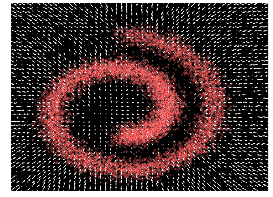
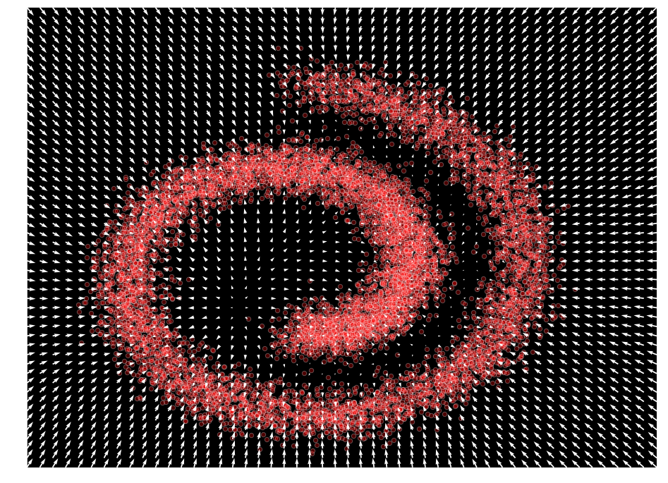
入力空間に渡り出力値をプロットすることにより、私たちのモデルが $\mathcal{F}_{\theta}(\mathbf{x}) \approx \nabla_x \log p(x)$ を表すことを学習したことを観測できます。

def plot_gradients(model, data, plot_scatter=True):
    xx = np.stack(np.meshgrid(np.linspace(-1.5, 2.0, 50), np.linspace(-1.5, 2.0, 50)), axis=-1).reshape(-1, 2)
    scores = model(torch.tensor(xx).float()).detach()
    scores_norm = np.linalg.norm(scores, axis=-1, ord=2, keepdims=True)
    scores_log1p = scores / (scores_norm + 1e-9) * np.log1p(scores_norm)
    # Perform the plots
    plt.figure(figsize=(16,12))
    if (plot_scatter):
        plt.scatter(*data, alpha=0.3, color='red', edgecolor='white', s=40)
    plt.quiver(*xx.T, *scores_log1p.T, width=0.002, color='white')
    plt.xlim(-1.5, 2.0)
    plt.ylim(-1.5, 2.0)
plot_gradients(model, data)

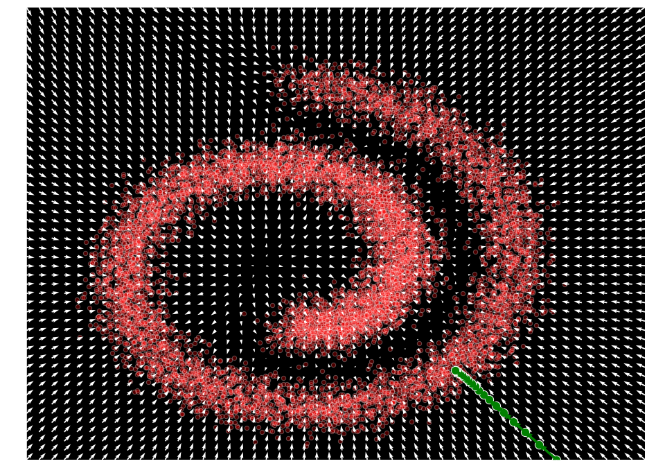
ランジュバン動力学

訓練後、モデルは $\mathcal{F}_{\theta}(\mathbf{x}) \approx \nabla_x \log p(x)$ であるように確率の勾配の近似を生成できるようになりました。従って、これを使用して、初期サンプル $\mathbf{x}_{0} \sim \mathcal{N}(\mathbf{0},\mathbf{I})$ を使用することにより与えられたポイントから単純な勾配上昇に依存して、それから $p(\mathbf{x})$ の局所最大値を見つけるために勾配情報を使用してデータを生成することができます。

\[
\mathbf{x}_{t + 1} = \mathbf{x}_t + \epsilon \nabla_{\mathbf{x}_t} log p(\mathbf{x}_t)
\]

ここで $\epsilon$ は勾配の方向に取るステップのサイズです (学習率に類似) 。

def sample_simple(model, x, n_steps=20, eps=1e-3):
    x_sequence = [x.unsqueeze(0)]
    for s in range(n_steps):
        x = x + eps * model(x)
        x_sequence.append(x.unsqueeze(0))
    return torch.cat(x_sequence)

x = torch.Tensor([1.5, -1.5])
samples = sample_simple(model, x).detach()
plot_gradients(model, data)
plt.scatter(samples[:, 0], samples[:, 1], color='green', edgecolor='white', s=150)
# draw arrows for each  step
deltas = (samples[1:] - samples[:-1])
deltas = deltas - deltas / np.linalg.norm(deltas, keepdims=True, axis=-1) * 0.04
for i, arrow in enumerate(deltas):
    plt.arrow(samples[i,0], samples[i,1], arrow[0], arrow[1], width=1e-4, head_width=2e-2, color="green", linewidth=3)

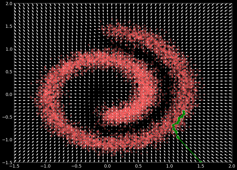
けれども、前の手順は $\mathbf{x} \sim p(\mathbf{x})$ からの真のサンプルを生成していません。そのようなサンプルを取得するために、ランジュバン動力学の特殊なケースに頼ることができます。この場合、ランジュバン動力学は、$\nabla_{\mathbf{x}} \log p(\mathbf{x})$ だけに依存して密度 $p(\mathbf{x})$ から真のサンプルを生成することができます。サンプリングは、次を再帰的に適用することにより、MCMC アプローチに非常に似た方法で定義されます :

\[
\mathbf{x}_{t + 1} = \mathbf{x}_t + \frac{\epsilon}{2} \nabla_{\mathbf{x}_t} log p(\mathbf{x}_t) + \sqrt{\epsilon} \mathbf{z}_{t}
\]

ここで $\mathbf{z}_{t}\sim \mathcal{N}(\mathbf{0},\mathbf{I})$ です。$\epsilon \rightarrow 0, t \rightarrow \inf$ のもとで、$\mathbf{x}_t$ は $p(\mathbf{x})$ からの正確なサンプルに収束することが Welling et al. (2011) で示されています。これがスコアベース生成モデリング・アプローチの裏の主要なアイデアです。

このサンプリング手順を実装するためには、$p(\mathbf{x})$ から真のサンプルを得るために、再度 $\mathbf{x}_{0} \sim \mathcal{N}(\mathbf{0},\mathbf{I})$ から始めて、段階的に各ステップで $\epsilon \rightarrow 0$ をアニールすることができます。

def sample_langevin(model, x, n_steps=10, eps=1e-2, decay=.9, temperature=1.0):
    x_sequence = [x.unsqueeze(0)]
    for s in range(n_steps):
        z_t = torch.rand(x.size())
        x = x + (eps / 2) * model(x) + (np.sqrt(eps) * temperature * z_t)
        x_sequence.append(x.unsqueeze(0))
        eps *= decay
    return torch.cat(x_sequence)

x = torch.Tensor([1.5, -1.5])
samples = sample_langevin(model, x).detach()
plot_gradients(model, data)
plt.scatter(samples[:, 0], samples[:, 1], color='green', edgecolor='white', s=150)
# draw arrows for each mcmc step
deltas = (samples[1:] - samples[:-1])
deltas = deltas - deltas / np.linalg.norm(deltas, keepdims=True, axis=-1) * 0.04
for i, arrow in enumerate(deltas):
    plt.arrow(samples[i,0], samples[i,1], arrow[0], arrow[1], width=1e-4, head_width=2e-2, color="green", linewidth=3)

Sliced スコアマッチング

この損失を持つ前に定義されたスコアマッチングは、$\text{ tr}\left( \nabla_{\mathbf{x}} \mathcal{F}_{\theta}(\mathbf{x}) \right)$ の計算量ゆえに、高次元データにも深層ネットワークにもスケーラブルではありません。実際に、ヤコビアンの計算量は $O(N^2 + N)$ 演算で、そのため前のコードで提案された最適化解法によってさえも高次元問題に対しては適しません。比較的最近、Song et al. [7] はスコアマッチングの $\text{ tr}\left( \nabla_{\mathbf{x}} \mathcal{F}_{\theta}(\mathbf{x}) \right)$ の計算を近似するためにランダムな射影を使用することを提案しました。sliced スコアマッチングと呼ばれるこのアプローチは最適化 objective を以下で置き換えることを可能にします :

\[
E_{\mathbf{v} \sim \mathcal{N}(0, 1)} E_{\mathbf{x} \sim p(\mathbf{x})} \left[ \mathbf{v}^T \nabla_{\mathbf{x}} \mathcal{F}_{\theta}(\mathbf{x}) \mathbf{v} + \frac{1}{2} \left\Vert \mathbf{v}^T \mathcal{F}_{\theta}(\mathbf{x}) \right\lVert_2^2 \right]
,
\]

ここで $\mathbf{v} \sim \mathcal{N}(0, 1)$ は正規分布のベクトルのセットです。これは計算的に効率的な forward モードの自動微分を使用して計算できることを彼らは示しました。この損失は以下のように実装できます (ここで再度ノルムを最初に、それからヤコビアン損失を計算します) :

def sliced_score_matching(model, samples):
    samples.requires_grad_(True)
    # Construct random vectors
    vectors = torch.randn_like(samples)
    vectors = vectors / torch.norm(vectors, dim=-1, keepdim=True)
    # Compute the optimized vector-product jacobian
    logp, jvp = autograd.functional.jvp(model, samples, vectors, create_graph=True)
    # Compute the norm loss
    norm_loss = (logp * vectors) ** 2 / 2.
    # Compute the Jacobian loss
    v_jvp = jvp * vectors
    jacob_loss = v_jvp
    loss = jacob_loss + norm_loss
    return loss.mean(-1).mean(-1)

前のように、サンプルのセットが与えられたときこの損失の単純な最適化を実行できます。

# Our approximation model
model = nn.Sequential(
    nn.Linear(2, 128), nn.Softplus(),
    nn.Linear(128, 128), nn.Softplus(),
    nn.Linear(128, 2)
)
# Create ADAM optimizer over our model
optimizer = optim.Adam(model.parameters(), lr=1e-3)
dataset = torch.tensor(data.T)[:1000].float()
for t in range(2000):
    # Compute the loss.
    loss = sliced_score_matching(model, dataset)
    # Before the backward pass, zero all of the network gradients
    optimizer.zero_grad()
    # Backward pass: compute gradient of the loss with respect to parameters
    loss.backward()
    # Calling the step function to update the parameters
    optimizer.step()
    # Print loss
    if ((t % 500) == 0):
        print(loss)

tensor(0.1118, grad_fn=<MeanBackward1>)
tensor(-1.0128, grad_fn=<MeanBackward1>)
tensor(-5.7355, grad_fn=<MeanBackward1>)
tensor(-8.0160, grad_fn=<MeanBackward1>)

前と同じ関数を頼りにして近似を確認できます。

plot_gradients(model, data)

ノイズ除去スコアマッチング

元々は、ノイズ除去スコアマッチングの考えは Vincent [3] によりノイズ除去オートエンコーダのコンテキストで議論されました。その場合、これはスコアマッチングの計算で $\nabla_{\mathbf{x}} \mathcal{F}_{\theta}(\mathbf{x})$ の使用を完全に除去することを可能にします。そのため、最初に与えられたノイズベクトルで入力ポイント $x$ を corrupt させることができて、これは分布 $q_{\sigma}(\tilde{\mathbf{x}}\mid\mathbf{x})$ になります。そして、この摂動されたデータ分布のスコアを推定するためにスコアマッチングが利用できます。$\mathcal{F}_{\theta}(\mathbf{x}) \approx \nabla_{\mathbf{x}} \log p(\mathbf{x})$ を近似する最適なネットワークは次の objective を最小化することにより見つけられることが [3] で示されています :

\[
E_{q_{\sigma}(\tilde{\mathbf{x}}\mid\mathbf{x})} E_{\mathbf{x} \sim p(\mathbf{x})} \left[ \left\Vert \mathcal{F}_{\theta}(\tilde{\mathbf{x}}) – \nabla_{\tilde{\mathbf{x}}} \log q_{\sigma}(\tilde{\mathbf{x}}\mid\mathbf{x}) \right\lVert_2^2 \right]
,
\]

けれども、$q_{\sigma}(\mathbf{x}) \approx p(\mathbf{x})$ を考慮するほどにノイズが十分に小さいときに限り、$\mathcal{F}_{\theta}(\mathbf{x}) = \nabla_{\mathbf{x}} \log q_{\sigma}(\mathbf{x}) \approx \nabla_{\mathbf{x}} \log p(\mathbf{x})$ が真であることに注意するべきです。[3], [8] で示されたように、ノイズ分布を $q_{\sigma}(\tilde{\mathbf{x}}\mid\mathbf{x})=\mathcal{N}(\tilde{\mathbf{x}}\mid\mathbf{x}, \sigma^{2}\mathbf{I})$ であるように選択する場合、$\nabla_{\tilde{\mathbf{x}}} \log q_{\sigma}(\tilde{\mathbf{x}}\mid\mathbf{x}) = \frac{\tilde{\mathbf{x}} – \mathbf{x}}{\sigma^{2}}$ を持ちます。従って、ノイズ除去スコアマッチング損失は単純に次になります :

\[
\mathcal{l}(\theta;\sigma) = E_{q_{\sigma}(\tilde{\mathbf{x}}\mid\mathbf{x})} E_{\mathbf{x} \sim p(\mathbf{x})} \left[ \left\Vert \mathcal{F}_{\theta}(\tilde{\mathbf{x}}) + \frac{\tilde{\mathbf{x}} – \mathbf{x}}{\sigma^{2}} \right\lVert_2^2 \right]
,
\]

ノイズ除去マッチング損失を以下のように実装できます :

def denoising_score_matching(scorenet, samples, sigma=0.01):
    perturbed_samples = samples + torch.randn_like(samples) * sigma
    target = - 1 / (sigma ** 2) * (perturbed_samples - samples)
    scores = scorenet(perturbed_samples)
    target = target.view(target.shape[0], -1)
    scores = scores.view(scores.shape[0], -1)
    loss = 1 / 2. * ((scores - target) ** 2).sum(dim=-1).mean(dim=0)
    return loss

前と同じモデルと optimizer に頼ります :

# Our approximation model
model = nn.Sequential(
    nn.Linear(2, 128), nn.Softplus(),
    nn.Linear(128, 128), nn.Softplus(),
    nn.Linear(128, 2)
)
# Create ADAM optimizer over our model
optimizer = optim.Adam(model.parameters(), lr=1e-3)
dataset = torch.tensor(data.T).float()
for t in range(5000):
    # Compute the loss.
    loss = denoising_score_matching(model, dataset)
    # Before the backward pass, zero all of the network gradients
    optimizer.zero_grad()
    # Backward pass: compute gradient of the loss with respect to parameters
    loss.backward()
    # Calling the step function to update the parameters
    optimizer.step()
    # Print loss
    if ((t % 1000) == 0):
        print(loss)

tensor(9778.1660, grad_fn=<MulBackward0>)
tensor(9862.8447, grad_fn=<MulBackward0>)
tensor(9976.3896, grad_fn=<MulBackward0>)
tensor(9933.9912, grad_fn=<MulBackward0>)
tensor(9779.1250, grad_fn=<MulBackward0>)

plot_gradients(model, data)

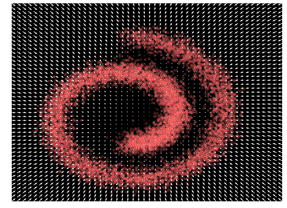
ノイズ条件付きスコアネットワーク

最近の論文で、Song と Ermon [8] はこれらのアイデアをもとに、ノイズ条件付きスコアネットワーク (NCSN) と呼ばれるスコアベースの生成フレームワークを開発しました。彼らは既存のスコアマッチング objective の幾つかの欠点をはっきりと示しました。最初に、データが多様体仮説に従うときノイズなしの (sliced) スコアマッチングの使用は矛盾があること、つまりノイズのない objective は分布が空間全体に広がるときだけ一貫性があることを示しました。2 番目に、低密度な領域はスコアマッチングとランジュバン動力学によるサンプリングの両者に対して困難さをもたらす可能性があることを示しました。

これらの問題に対処するため、多様体問題を回避するために摂動されたデータに頼り、しかしまた単一の条件付きスコアネットワークを訓練することにより総てのノイズレベルに対応したスコアを同時に推定することを提案しています。そのため、ノイズ分散 $\{\sigma_{i}\}_{i=1}^{L}$ の正値の幾何学的なシークエンスを考えます、$\sigma_{1}$ は多様体問題を軽減するために十分大きく取り、$\frac{\sigma_{1}}{\sigma_{2}} = \cdots = \frac{\sigma_{L-1}}{\sigma_{L}} > 1$ を満たします。目標は総ての摂動データ分布の勾配を推定するために条件付きネットワークを訓練することです、つまり :

\[
\forall \sigma \in \{\sigma_{i}\}_{i=1}^{L}, \mathcal{F}_{\theta}(\tilde{\mathbf{x}}, \sigma) \approx \nabla_{\mathbf{x}} \log q_{\sigma}(\mathbf{x})
\]

これを学習するネットワークはノイズ条件付きスコアネットワーク (NCSN) と呼ばれます。この最適化を行なうために、前に定義したノイズ除去スコアマッチング objective から始めます :

\[
\mathcal{l}(\theta;\sigma) = E_{q_{\sigma}(\tilde{\mathbf{x}}\mid\mathbf{x})} E_{\mathbf{x} \sim p(\mathbf{x})} \left[ \left\Vert \mathcal{F}_{\theta}(\tilde{\mathbf{x}}, \sigma) + \frac{\tilde{\mathbf{x}} – \mathbf{x}}{\sigma^{2}} \right\lVert_2^2 \right]
,
\]

これは単一のノイズレベルを扱うので、この objective は次のように単一の統合 objective を得るために組み合わせることができます :

\[
\mathcal{L}(\theta;\{\sigma_{i}\}_{i=1}^{L}) = \frac{1}{L} \sum_{i=1}^{L} \lambda(\sigma_{i})\mathcal{l}(\theta;\sigma_{i})
\]

ここで $\lambda(\sigma_{i}) > 0$ は $\sigma_{i}$ に依存する係数関数です。この objective は以下のように実装できます :

def anneal_dsm_score_estimation(model, samples, labels, sigmas, anneal_power=2.):
    used_sigmas = sigmas[labels].view(samples.shape[0], *([1] * len(samples.shape[1:])))
    perturbed_samples = samples + torch.randn_like(samples) * used_sigmas
    target = - 1 / (used_sigmas ** 2) * (perturbed_samples - samples)
    scores = model(perturbed_samples, labels)
    target = target.view(target.shape[0], -1)
    scores = scores.view(scores.shape[0], -1)
    loss = 1 / 2. * ((scores - target) ** 2).sum(dim=-1) * used_sigmas.squeeze() ** anneal_power
    return loss.mean(dim=0)

前の等式で見れたように、このモデルは条件付きネットワーク $\mathcal{F}_{\theta}(\tilde{\mathbf{x}}, \sigma_{i})$ を必要とします、これはまた入力として別のノイズレベル $\sigma_{i}$ を取ります。そして、それを構成するために前のモデルを再定義します :

import torch.nn.functional as F

class ConditionalLinear(nn.Module):
    def __init__(self, num_in, num_out, num_classes):
        super().__init__()
        self.num_out = num_out
        self.lin = nn.Linear(num_in, num_out)
        self.embed = nn.Embedding(num_classes, num_out)
        self.embed.weight.data.uniform_()

    def forward(self, x, y):
        out = self.lin(x)
        gamma = self.embed(y)
        out = gamma.view(-1, self.num_out) * out
        return out
    
class ConditionalModel(nn.Module):
    def __init__(self, num_classes):
        super().__init__()
        self.lin1 = ConditionalLinear(2, 128, num_classes)
        self.lin2 = ConditionalLinear(128, 128, num_classes)
        self.lin3 = nn.Linear(128, 2)
    
    def forward(self, x, y):
        x = F.softplus(self.lin1(x, y))
        x = F.softplus(self.lin2(x, y))
        return self.lin3(x)

最後に、前と同じ最適化を遂行できます :

sigma_begin = 1
sigma_end = 0.01
num_classes = 4
sigmas = torch.tensor(np.exp(np.linspace(np.log(sigma_begin), np.log(sigma_end), num_classes))).float()
# Our approximation model
model = ConditionalModel(num_classes)
dataset = torch.tensor(data.T).float()
# Create ADAM optimizer over our model
optimizer = optim.Adam(model.parameters(), lr=1e-3)
for t in range(5000):
    # Compute the loss.
    labels = torch.randint(0, len(sigmas), (dataset.shape[0],))
    loss = anneal_dsm_score_estimation(model, dataset, labels, sigmas)
    # Before the backward pass, zero all of the network gradients
    optimizer.zero_grad()
    # Backward pass: compute gradient of the loss with respect to parameters
    loss.backward()
    # Calling the step function to update the parameters
    optimizer.step()
    # Print loss
    if ((t % 1000) == 0):
        print(loss)

tensor(1.0319, grad_fn=<MeanBackward1>)
tensor(0.7983, grad_fn=<MeanBackward1>)
tensor(0.7847, grad_fn=<MeanBackward1>)
tensor(0.7673, grad_fn=<MeanBackward1>)
tensor(0.7460, grad_fn=<MeanBackward1>)

xx = np.stack(np.meshgrid(np.linspace(-1.5, 2.0, 50), np.linspace(-1.5, 2.0, 50)), axis=-1).reshape(-1, 2)
labels = torch.randint(0, len(sigmas), (xx.shape[0],))
scores = model(torch.tensor(xx).float(), labels).detach()
scores_norm = np.linalg.norm(scores, axis=-1, ord=2, keepdims=True)
scores_log1p = scores / (scores_norm + 1e-9) * np.log1p(scores_norm)
# Perform the plots
plt.figure(figsize=(16,12))
plt.scatter(*data, alpha=0.3, color='red', edgecolor='white', s=40)
plt.quiver(*xx.T, *scores_log1p.T, width=0.002, color='white')
plt.xlim(-1.5, 2.0)
plt.ylim(-1.5, 2.0);

xx = np.stack(np.meshgrid(np.linspace(-1.5, 2.0, 50), np.linspace(-1.5, 2.0, 50)), axis=-1).reshape(-1, 2)
labels = torch.ones(xx.shape[0]).long()
scores = model(torch.tensor(xx).float(), labels).detach()
scores_norm = np.linalg.norm(scores, axis=-1, ord=2, keepdims=True)
scores_log1p = scores / (scores_norm + 1e-9) * np.log1p(scores_norm)
# Perform the plots
plt.figure(figsize=(16,12))
plt.scatter(*data, alpha=0.3, color='red', edgecolor='white', s=40)
plt.quiver(*xx.T, *scores_log1p.T, width=0.002, color='white')
plt.xlim(-1.5, 2.0)
plt.ylim(-1.5, 2.0)

(-1.5, 2.0)

参考文献

以上

月	火	水	木	金	土	日
			1	2	3	4
5	6	7	8	9	10	11
12	13	14	15	16	17	18
19	20	21	22	23	24	25
26	27	28	29	30