Lightly 1.2 : Tutorials : 4. 衛星画像上の SimSiam の訓練 (翻訳/解説)

翻訳 : (株)クラスキャットセールスインフォメーション
作成日時 : 08/21/2022 (v1.2.27)

* 本ページは、Lightly の以下のドキュメントを翻訳した上で適宜、補足説明したものです：

Tutorials : Tutorial 4: Train SimSiam on Satellite Images

* サンプルコードの動作確認はしておりますが、必要な場合には適宜、追加改変しています。
* ご自由にリンクを張って頂いてかまいませんが、sales-info@classcat.com までご一報いただけると嬉しいです。

クラスキャット人工知能研究開発支援サービス

◆ クラスキャットは人工知能・テレワークに関する各種サービスを提供しています。お気軽にご相談ください :

人工知能研究開発支援
1. 人工知能研修サービス(経営者層向けオンサイト研修)
2. テクニカルコンサルティングサービス
3. 実証実験(プロトタイプ構築)
4. アプリケーションへの実装
人工知能研修サービス
PoC(概念実証)を失敗させないための支援

◆ 人工知能とビジネスをテーマに WEB セミナーを定期的に開催しています。スケジュール。

お住まいの地域に関係なく Web ブラウザからご参加頂けます。事前登録 が必要ですのでご注意ください。

◆ お問合せ : 本件に関するお問い合わせ先は下記までお願いいたします。

株式会社クラスキャット セールス・マーケティング本部セールス・インフォメーション
sales-info@classcat.com ; Web: www.classcat.com ; ClassCatJP

Lightly 1.2 : Tutorials : 4. 衛星画像上の SimSiam の訓練

このチュートリアルでは、イタリアの衛星画像のセットで従来の PyTorch スタイルで SimSiam モデルを訓練します。生成された埋め込みが生データの調査とより良い理解のためにどのように使用できるかを紹介します。

論文 Exploring Simple Siamese Representation Learning でモデルを調べることができます。

イタリアの ESA Sentinel-2 satellite (監視衛星) からの衛星画像のデータセットを使用していきます。興味があれば、コペルニクス Open Access ハブから独自データを取得できます。元の画像は巨大なサイズなので小さいタイルに切り抜かれていて、データセットは過剰な海の画像を防ぐために平均 RGB カラー値の単純なクラスタリングに基づいてバランスが取られています。

このチュートリアルで学習するものは :

SimSiam モデルを扱う方法
PyTorch を使用して自己教師あり学習を行なう方法
埋め込みが壊れていないか確認する方法

インポート

このチュートリアルに必要な Python フレームワークをインポートします。

import math
import torch
import torch.nn as nn
import torchvision
import numpy as np
import lightly
from lightly.models.modules.heads import SimSiamPredictionHead
from lightly.models.modules.heads import SimSiamProjectionHead

Configuration

実験のために幾つかの設定パラメータを設定します。

256 のバッチサイズと入力解像度のデフォルト設定は 16GB の GPU メモリを必要とします。

num_workers = 8
batch_size = 128
seed = 1
epochs = 50
input_size = 256

# dimension of the embeddings
num_ftrs = 512
# dimension of the output of the prediction and projection heads
out_dim = proj_hidden_dim = 512
# the prediction head uses a bottleneck architecture
pred_hidden_dim = 128

実験のためのシードとデータへのパスを設定しましょう。

# seed torch and numpy
torch.manual_seed(0)
np.random.seed(0)

# set the path to the dataset
path_to_data = '/datasets/sentinel-2-italy-v1/'

データ増強とローダのセットアップ

衛星画像を扱っているので、水平と垂直反転とランダム回転変換を使用することは意味があります。水の色の僅かの変化に関してモデルの普遍性を学習するために弱いカラージッターを適用します。

# define the augmentations for self-supervised learning
collate_fn = lightly.data.ImageCollateFunction(
    input_size=input_size,
    # require invariance to flips and rotations
    hf_prob=0.5,
    vf_prob=0.5,
    rr_prob=0.5,
    # satellite images are all taken from the same height
    # so we use only slight random cropping
    min_scale=0.5,
    # use a weak color jitter for invariance w.r.t small color changes
    cj_prob=0.2,
    cj_bright=0.1,
    cj_contrast=0.1,
    cj_hue=0.1,
    cj_sat=0.1,
)

# create a lightly dataset for training, since the augmentations are handled
# by the collate function, there is no need to apply additional ones here
dataset_train_simsiam = lightly.data.LightlyDataset(
    input_dir=path_to_data
)

# create a dataloader for training
dataloader_train_simsiam = torch.utils.data.DataLoader(
    dataset_train_simsiam,
    batch_size=batch_size,
    shuffle=True,
    collate_fn=collate_fn,
    drop_last=True,
    num_workers=num_workers
)

# create a torchvision transformation for embedding the dataset after training
# here, we resize the images to match the input size during training and apply
# a normalization of the color channel based on statistics from imagenet
test_transforms = torchvision.transforms.Compose([
    torchvision.transforms.Resize((input_size, input_size)),
    torchvision.transforms.ToTensor(),
    torchvision.transforms.Normalize(
        mean=lightly.data.collate.imagenet_normalize['mean'],
        std=lightly.data.collate.imagenet_normalize['std'],
    )
])

# create a lightly dataset for embedding
dataset_test = lightly.data.LightlyDataset(
    input_dir=path_to_data,
    transform=test_transforms
)

# create a dataloader for embedding
dataloader_test = torch.utils.data.DataLoader(
    dataset_test,
    batch_size=batch_size,
    shuffle=False,
    drop_last=False,
    num_workers=num_workers
)

SimSiam モデルの作成

ResNet バックボーンを作成して分類ヘッドを除去します。

class SimSiam(nn.Module):
    def __init__(
        self, backbone, num_ftrs, proj_hidden_dim, pred_hidden_dim, out_dim
    ):
        super().__init__()
        self.backbone = backbone
        self.projection_head = SimSiamProjectionHead(
            num_ftrs, proj_hidden_dim, out_dim
        )
        self.prediction_head = SimSiamPredictionHead(
            out_dim, pred_hidden_dim, out_dim
        )

    def forward(self, x):
        # get representations
        f = self.backbone(x).flatten(start_dim=1)
        # get projections
        z = self.projection_head(f)
        # get predictions
        p = self.prediction_head(z)
        # stop gradient
        z = z.detach()
        return z, p


# we use a pretrained resnet for this tutorial to speed
# up training time but you can also train one from scratch
resnet = torchvision.models.resnet18()
backbone = nn.Sequential(*list(resnet.children())[:-1])
model = SimSiam(backbone, num_ftrs, proj_hidden_dim, pred_hidden_dim, out_dim)

SimSiam は対称的な負のコサイン類似度損失を使用し、従ってネガティブサンプルを必要としません。criterion と optimizer を構築します。

# SimSiam uses a symmetric negative cosine similarity loss
criterion = lightly.loss.NegativeCosineSimilarity()

# scale the learning rate
lr = 0.05 * batch_size / 256
# use SGD with momentum and weight decay
optimizer = torch.optim.SGD(
    model.parameters(),
    lr=lr,
    momentum=0.9,
    weight_decay=5e-4
)

SimSiam の訓練

SimSiam モデルを訓練するため、従来の PyTorch 訓練ループを使用できます : 総てのエポックに対して、訓練データの総てのバッチに渡りイテレートし、総ての画像の 2 つの変換を抽出し、それらをモデルを通し、そして損失を計算します。そして、単純に optimizer で重みを更新します。勾配をリセットするのを忘れないでください！

SimSiam はネガティブサンプルを必要としないので、モデルの出力が単一の方向に collapse していないか確認するのは良い考えです。このためには L2 正規化出力ベクトルの標準偏差を単純に確認できます。それが出力次元の平方根で除算したものに近ければ、総てが上手くいっています (このアイデアについてここで読んで調べることができます)。

device = 'cuda' if torch.cuda.is_available() else 'cpu'
model.to(device)

avg_loss = 0.
avg_output_std = 0.
for e in range(epochs):

    for (x0, x1), _, _ in dataloader_train_simsiam:

        # move images to the gpu
        x0 = x0.to(device)
        x1 = x1.to(device)

        # run the model on both transforms of the images
        # we get projections (z0 and z1) and
        # predictions (p0 and p1) as output
        z0, p0 = model(x0)
        z1, p1 = model(x1)

        # apply the symmetric negative cosine similarity
        # and run backpropagation
        loss = 0.5 * (criterion(z0, p1) + criterion(z1, p0))
        loss.backward()

        optimizer.step()
        optimizer.zero_grad()

        # calculate the per-dimension standard deviation of the outputs
        # we can use this later to check whether the embeddings are collapsing
        output = p0.detach()
        output = torch.nn.functional.normalize(output, dim=1)

        output_std = torch.std(output, 0)
        output_std = output_std.mean()

        # use moving averages to track the loss and standard deviation
        w = 0.9
        avg_loss = w * avg_loss + (1 - w) * loss.item()
        avg_output_std = w * avg_output_std + (1 - w) * output_std.item()

    # the level of collapse is large if the standard deviation of the l2
    # normalized output is much smaller than 1 / sqrt(dim)
    collapse_level = max(0., 1 - math.sqrt(out_dim) * avg_output_std)
    # print intermediate results
    print(f'[Epoch {e:3d}] '
        f'Loss = {avg_loss:.2f} | '
        f'Collapse Level: {collapse_level:.2f} / 1.00')

[Epoch   0] Loss = -0.85 | Collapse Level: 0.17 / 1.00
[Epoch   1] Loss = -0.86 | Collapse Level: 0.14 / 1.00
[Epoch   2] Loss = -0.86 | Collapse Level: 0.12 / 1.00
[Epoch   3] Loss = -0.86 | Collapse Level: 0.10 / 1.00
[Epoch   4] Loss = -0.86 | Collapse Level: 0.11 / 1.00
[Epoch   5] Loss = -0.88 | Collapse Level: 0.11 / 1.00
[Epoch   6] Loss = -0.88 | Collapse Level: 0.10 / 1.00
[Epoch   7] Loss = -0.88 | Collapse Level: 0.09 / 1.00
[Epoch   8] Loss = -0.89 | Collapse Level: 0.09 / 1.00
[Epoch   9] Loss = -0.88 | Collapse Level: 0.08 / 1.00
[Epoch  10] Loss = -0.90 | Collapse Level: 0.09 / 1.00
[Epoch  11] Loss = -0.90 | Collapse Level: 0.09 / 1.00
[Epoch  12] Loss = -0.90 | Collapse Level: 0.09 / 1.00
[Epoch  13] Loss = -0.89 | Collapse Level: 0.11 / 1.00
[Epoch  14] Loss = -0.89 | Collapse Level: 0.12 / 1.00
[Epoch  15] Loss = -0.89 | Collapse Level: 0.12 / 1.00
[Epoch  16] Loss = -0.90 | Collapse Level: 0.13 / 1.00
[Epoch  17] Loss = -0.89 | Collapse Level: 0.14 / 1.00
[Epoch  18] Loss = -0.89 | Collapse Level: 0.14 / 1.00
[Epoch  19] Loss = -0.90 | Collapse Level: 0.14 / 1.00
[Epoch  20] Loss = -0.91 | Collapse Level: 0.14 / 1.00
[Epoch  21] Loss = -0.90 | Collapse Level: 0.13 / 1.00
[Epoch  22] Loss = -0.91 | Collapse Level: 0.14 / 1.00
[Epoch  23] Loss = -0.91 | Collapse Level: 0.12 / 1.00
[Epoch  24] Loss = -0.91 | Collapse Level: 0.12 / 1.00
[Epoch  25] Loss = -0.92 | Collapse Level: 0.13 / 1.00
[Epoch  26] Loss = -0.92 | Collapse Level: 0.14 / 1.00
[Epoch  27] Loss = -0.92 | Collapse Level: 0.14 / 1.00
[Epoch  28] Loss = -0.92 | Collapse Level: 0.13 / 1.00
[Epoch  29] Loss = -0.93 | Collapse Level: 0.13 / 1.00
[Epoch  30] Loss = -0.92 | Collapse Level: 0.14 / 1.00
[Epoch  31] Loss = -0.93 | Collapse Level: 0.14 / 1.00
[Epoch  32] Loss = -0.94 | Collapse Level: 0.13 / 1.00
[Epoch  33] Loss = -0.92 | Collapse Level: 0.13 / 1.00
[Epoch  34] Loss = -0.94 | Collapse Level: 0.14 / 1.00
[Epoch  35] Loss = -0.93 | Collapse Level: 0.12 / 1.00
[Epoch  36] Loss = -0.93 | Collapse Level: 0.12 / 1.00
[Epoch  37] Loss = -0.93 | Collapse Level: 0.11 / 1.00
[Epoch  38] Loss = -0.94 | Collapse Level: 0.10 / 1.00
[Epoch  39] Loss = -0.94 | Collapse Level: 0.10 / 1.00
[Epoch  40] Loss = -0.93 | Collapse Level: 0.09 / 1.00
[Epoch  41] Loss = -0.93 | Collapse Level: 0.09 / 1.00
[Epoch  42] Loss = -0.94 | Collapse Level: 0.09 / 1.00
[Epoch  43] Loss = -0.93 | Collapse Level: 0.07 / 1.00
[Epoch  44] Loss = -0.93 | Collapse Level: 0.07 / 1.00
[Epoch  45] Loss = -0.94 | Collapse Level: 0.06 / 1.00
[Epoch  46] Loss = -0.93 | Collapse Level: 0.06 / 1.00
[Epoch  47] Loss = -0.94 | Collapse Level: 0.05 / 1.00
[Epoch  48] Loss = -0.93 | Collapse Level: 0.05 / 1.00
[Epoch  49] Loss = -0.94 | Collapse Level: 0.05 / 1.00

データセットに画像を埋め込むには、テストデータローダに対して単純に反復して画像をモデルバックボーンに供給します。この部分については勾配を確実に無効にしてください。

embeddings = []
filenames = []

# disable gradients for faster calculations
model.eval()
with torch.no_grad():
    for i, (x, _, fnames) in enumerate(dataloader_test):
        # move the images to the gpu
        x = x.to(device)
        # embed the images with the pre-trained backbone
        y = model.backbone(x).flatten(start_dim=1)
        # store the embeddings and filenames in lists
        embeddings.append(y)
        filenames = filenames + list(fnames)

# concatenate the embeddings and convert to numpy
embeddings = torch.cat(embeddings, dim=0)
embeddings = embeddings.cpu().numpy()

散布図と最近傍

埋め込みを持ったので、データを散布図で可視化できます。更に、幾つかのサンプル画像の最近傍も調査します。

最初のステップとして、幾つかの追加のインポートを行います。

# for plotting
import os
from PIL import Image

import matplotlib.pyplot as plt
import matplotlib.offsetbox as osb
from matplotlib import rcParams as rcp

# for resizing images to thumbnails
import torchvision.transforms.functional as functional

# for clustering and 2d representations
from sklearn import random_projection

次に、UMAP を使用して埋め込みを変換してそれらを [0, 1] 四方に収まるように再スケールします。

# for the scatter plot we want to transform the images to a two-dimensional
# vector space using a random Gaussian projection
projection = random_projection.GaussianRandomProjection(n_components=2)
embeddings_2d = projection.fit_transform(embeddings)

# normalize the embeddings to fit in the [0, 1] square
M = np.max(embeddings_2d, axis=0)
m = np.min(embeddings_2d, axis=0)
embeddings_2d = (embeddings_2d - m) / (M - m)

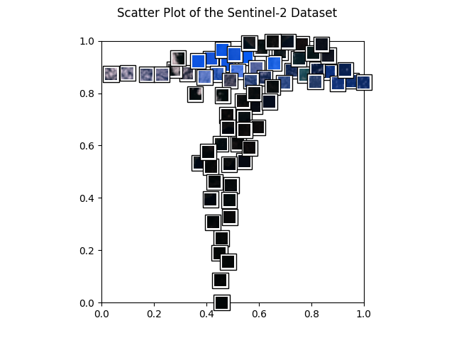
データセットの素敵な散布図から始めましょう！下のヘルパー関数で作成します。

def get_scatter_plot_with_thumbnails():
    """Creates a scatter plot with image overlays.
    """
    # initialize empty figure and add subplot
    fig = plt.figure()
    fig.suptitle('Scatter Plot of the Sentinel-2 Dataset')
    ax = fig.add_subplot(1, 1, 1)
    # shuffle images and find out which images to show
    shown_images_idx = []
    shown_images = np.array([[1., 1.]])
    iterator = [i for i in range(embeddings_2d.shape[0])]
    np.random.shuffle(iterator)
    for i in iterator:
        # only show image if it is sufficiently far away from the others
        dist = np.sum((embeddings_2d[i] - shown_images) ** 2, 1)
        if np.min(dist) < 2e-3:
            continue
        shown_images = np.r_[shown_images, [embeddings_2d[i]]]
        shown_images_idx.append(i)

    # plot image overlays
    for idx in shown_images_idx:
        thumbnail_size = int(rcp['figure.figsize'][0] * 2.)
        path = os.path.join(path_to_data, filenames[idx])
        img = Image.open(path)
        img = functional.resize(img, thumbnail_size)
        img = np.array(img)
        img_box = osb.AnnotationBbox(
            osb.OffsetImage(img, cmap=plt.cm.gray_r),
            embeddings_2d[idx],
            pad=0.2,
        )
        ax.add_artist(img_box)

    # set aspect ratio
    ratio = 1. / ax.get_data_ratio()
    ax.set_aspect(ratio, adjustable='box')


# get a scatter plot with thumbnail overlays
get_scatter_plot_with_thumbnails()

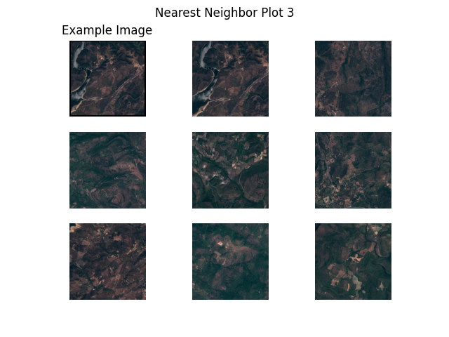
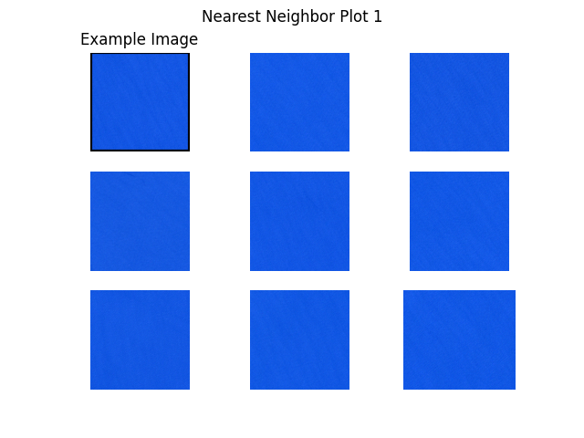
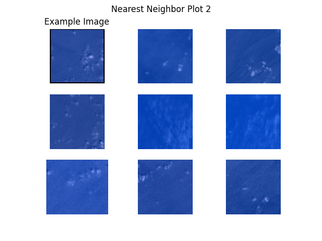
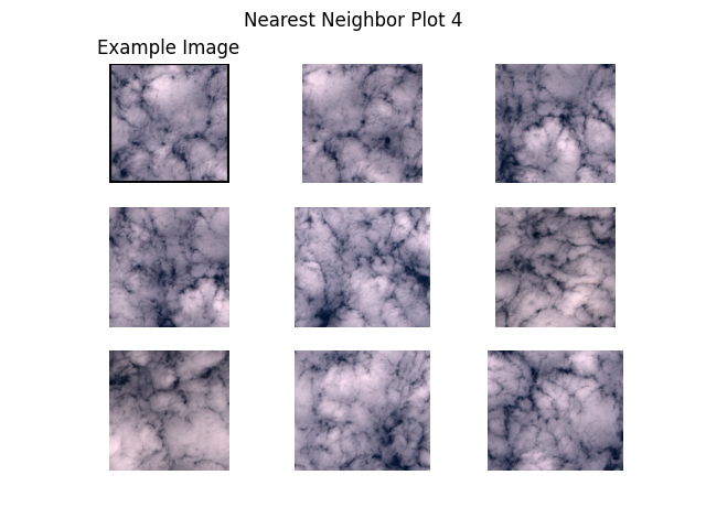
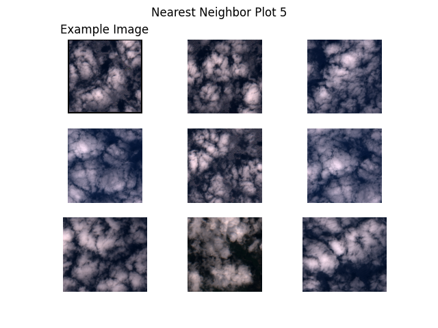
次に、サンプル画像とそれらの最近傍をプロットします (上で生成された埋め込みから計算します)。これは、(幾つかのサンプルが既に利用可能な) 特定のタイプのより多くの画像を見つけるための非常に単純なアプローチです。例えば、データのサブセットが既にラベル付けされて画像の一つのクラスが明らかに少ないとき、ラベル付けされていないデータからこのクラスのより多くの画像を容易に問い合わせることができます。

仕事を始めましょう！プロットは下で示されます。

example_images = [
    'S2B_MSIL1C_20200526T101559_N0209_R065_T31TGE/tile_00154.png', # water 1
    'S2B_MSIL1C_20200526T101559_N0209_R065_T32SLJ/tile_00527.png', # water 2
    'S2B_MSIL1C_20200526T101559_N0209_R065_T32TNL/tile_00556.png', # land
    'S2B_MSIL1C_20200526T101559_N0209_R065_T31SGD/tile_01731.png', # clouds 1
    'S2B_MSIL1C_20200526T101559_N0209_R065_T32SMG/tile_00238.png', # clouds 2
]


def get_image_as_np_array(filename: str):
    """Loads the image with filename and returns it as a numpy array.

    """
    img = Image.open(filename)
    return np.asarray(img)


def get_image_as_np_array_with_frame(filename: str, w: int = 5):
    """Returns an image as a numpy array with a black frame of width w.

    """
    img = get_image_as_np_array(filename)
    ny, nx, _ = img.shape
    # create an empty image with padding for the frame
    framed_img = np.zeros((w + ny + w, w + nx + w, 3))
    framed_img = framed_img.astype(np.uint8)
    # put the original image in the middle of the new one
    framed_img[w:-w, w:-w] = img
    return framed_img


def plot_nearest_neighbors_3x3(example_image: str, i: int):
    """Plots the example image and its eight nearest neighbors.

    """
    n_subplots = 9
    # initialize empty figure
    fig = plt.figure()
    fig.suptitle(f"Nearest Neighbor Plot {i + 1}")
    #
    example_idx = filenames.index(example_image)
    # get distances to the cluster center
    distances = embeddings - embeddings[example_idx]
    distances = np.power(distances, 2).sum(-1).squeeze()
    # sort indices by distance to the center
    nearest_neighbors = np.argsort(distances)[:n_subplots]
    # show images
    for plot_offset, plot_idx in enumerate(nearest_neighbors):
        ax = fig.add_subplot(3, 3, plot_offset + 1)
        # get the corresponding filename
        fname = os.path.join(path_to_data, filenames[plot_idx])
        if plot_offset == 0:
            ax.set_title(f"Example Image")
            plt.imshow(get_image_as_np_array_with_frame(fname))
        else:
            plt.imshow(get_image_as_np_array(fname))
        # let's disable the axis
        plt.axis("off")


# show example images for each cluster
for i, example_image in enumerate(example_images):
    plot_nearest_neighbors_3x3(example_image, i)

以上

2022年8月
月	火	水	木	金	土	日
1	2	3	4	5	6	7
8	9	10	11	12	13	14
15	16	17	18	19	20	21
22	23	24	25	26	27	28
29	30	31

Lightly 1.2 : Tutorials : 4. 衛星画像 上の SimSiam の訓練 (翻訳/解説)

Lightly 1.2 : Tutorials : 4. 衛星画像 上の SimSiam の訓練