MONAI 0.8 : MedNIST デモ (画像分類チュートリアル) (翻訳/解説)

翻訳 : (株)クラスキャット セールスインフォメーション
作成日時 : 12/31/2021 (0.8.0)

* 本ページは、MONAI の以下のドキュメントを翻訳した上で適宜、補足説明したものです：

• Image Classification Tutorial with the MedNIST Dataset

* サンプルコードの動作確認はしておりますが、必要な場合には適宜、追加改変しています。
* ご自由にリンクを張って頂いてかまいませんが、sales-info@classcat.com までご一報いただけると嬉しいです。

 

 

 

MONAI 0.8 : MedNIST デモ (画像分類チュートリアル)

イントロダクション

このチュートリアルでは、MedNIST データセットに基づいて end-to-end な訓練と評価サンプルを紹介します。以下のステップで進めます :

• 訓練とテストのための MONAI データセットを作成します。
• データの前処理のために MONAI 変換を使用します。
• 分類タスクのために MONAI から DenseNet を使用します。
• PyTorch プログラムでモデルを訓練します。
• テストデータセットで評価します。

 

データセットの取得

MedNIST データセットは TCIA, RSNA Bone Age チャレンジ と NIH Chest X-ray データセット からの様々なセットから集められました。

データセットは Dr. Bradley J. Erickson M.D., Ph.D. (Department of Radiology, Mayo Clinic) のお陰により Creative Commons CC BY-SA 4.0 ライセンス のもとで利用可能になっています。MedNIST データセットを使用する場合、出典を明示してください、e.g. https://github.com/Project-MONAI/tutorials/blob/master/2d_classification/mednist_tutorial.ipynb。

以下のコマンドはデータセット (~ 60MB) をダウンロードして unzip します。

!wget -q https://www.dropbox.com/s/5wwskxctvcxiuea/MedNIST.tar.gz

# unzip the '.tar.gz' file to the current directory
import tarfile
datafile = tarfile.open("MedNIST.tar.gz")
datafile.extractall()
datafile.close()

MONAI をインストールします :

!pip install -q "monai-weekly[gdown, nibabel, tqdm, itk]"

import os
import shutil
import tempfile
import matplotlib.pyplot as plt
from PIL import Image
import torch
import numpy as np
from sklearn.metrics import classification_report

from monai.apps import download_and_extract
from monai.config import print_config
from monai.metrics import ROCAUCMetric
from monai.networks.nets import DenseNet121
from monai.transforms import (
    Activations,
    AddChannel,
    AsDiscrete,
    Compose,
    LoadImage,
    RandFlip,
    RandRotate,
    RandZoom,
    ScaleIntensity,
    ToTensor,
)
from monai.data import Dataset, DataLoader
from monai.utils import set_determinism

print_config()

MONAI version: 0.8.dev2147
Numpy version: 1.19.5
Pytorch version: 1.10.0+cu111
MONAI flags: HAS_EXT = False, USE_COMPILED = False
MONAI rev id: 356ba3f25350e785387113684d6d2f4317a0f458

Optional dependencies:
Pytorch Ignite version: NOT INSTALLED or UNKNOWN VERSION.
Nibabel version: 3.0.2
scikit-image version: 0.18.3
Pillow version: 7.1.2
Tensorboard version: 2.7.0
gdown version: 3.6.4
TorchVision version: 0.11.1+cu111
tqdm version: 4.62.3
lmdb version: 0.99
psutil version: 5.4.8
pandas version: 1.1.5
einops version: NOT INSTALLED or UNKNOWN VERSION.
transformers version: NOT INSTALLED or UNKNOWN VERSION.
mlflow version: NOT INSTALLED or UNKNOWN VERSION.

For details about installing the optional dependencies, please visit:
    https://docs.monai.io/en/latest/installation.html#installing-the-recommended-dependencies

 

データセットフォルダから画像ファイル名を読む

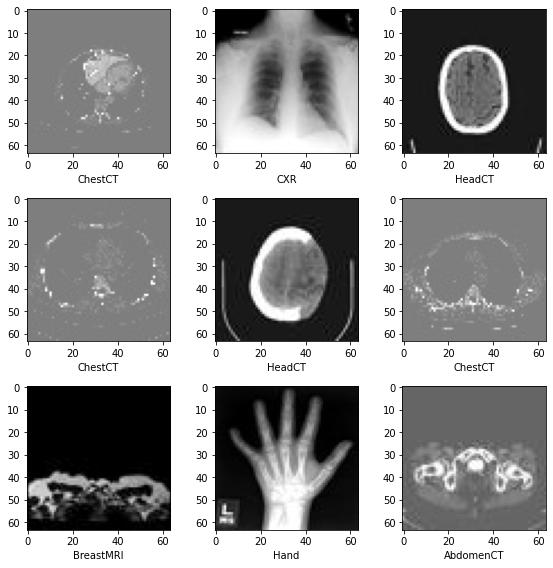
最初に、データセットファイルをチェックして幾つかの統計情報を示します。データセットには 6 つのフォルダがあります : Hand, AbdomenCT, CXR, ChestCT, BreastMRI, HeadCT, これらは分類モデルを訓練するラベルとして使用されるべきです。

data_dir = './MedNIST/'
class_names = sorted([x for x in os.listdir(data_dir) if os.path.isdir(os.path.join(data_dir, x))])
num_class = len(class_names)
image_files = [[os.path.join(data_dir, class_name, x) 
                for x in os.listdir(os.path.join(data_dir, class_name))] 
               for class_name in class_names]
image_file_list = []
image_label_list = []
for i, class_name in enumerate(class_names):
    image_file_list.extend(image_files[i])
    image_label_list.extend([i] * len(image_files[i]))
num_total = len(image_label_list)
image_width, image_height = Image.open(image_file_list[0]).size

print('Total image count:', num_total)
print("Image dimensions:", image_width, "x", image_height)
print("Label names:", class_names)
print("Label counts:", [len(image_files[i]) for i in range(num_class)])

Total image count: 58954
Image dimensions: 64 x 64
Label names: ['AbdomenCT', 'BreastMRI', 'CXR', 'ChestCT', 'Hand', 'HeadCT']
Label counts: [10000, 8954, 10000, 10000, 10000, 10000]

 

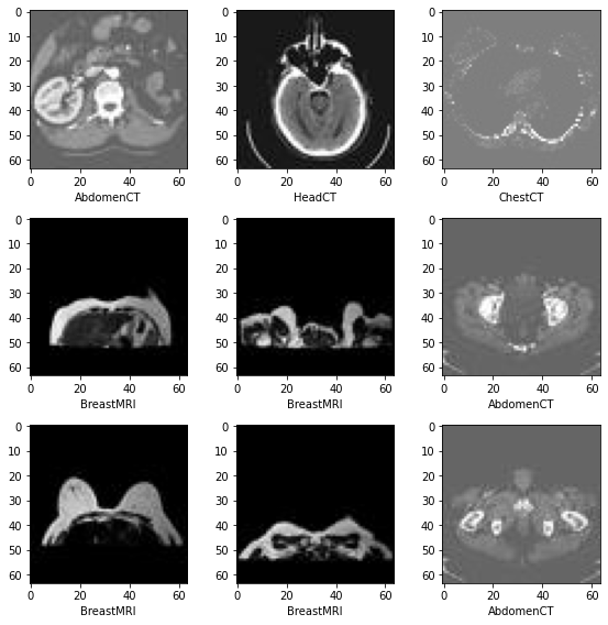
データセットからランダムに選択されたサンプルを可視化する

plt.subplots(3, 3, figsize=(8, 8))
for i,k in enumerate(np.random.randint(num_total, size=9)):
    im = Image.open(image_file_list[k])
    arr = np.array(im)
    plt.subplot(3, 3, i + 1)
    plt.xlabel(class_names[image_label_list[k]])
    plt.imshow(arr, cmap='gray', vmin=0, vmax=255)
plt.tight_layout()
plt.show()

 

訓練、検証とテストデータリストの準備

データセットの 10% を検証用に 10% をテスト用にランダムに選択します。

valid_frac, test_frac = 0.1, 0.1
trainX, trainY = [], []
valX, valY = [], []
testX, testY = [], []

for i in range(num_total):
    rann = np.random.random()
    if rann < valid_frac:
        valX.append(image_file_list[i])
        valY.append(image_label_list[i])
    elif rann < test_frac + valid_frac:
        testX.append(image_file_list[i])
        testY.append(image_label_list[i])
    else:
        trainX.append(image_file_list[i])
        trainY.append(image_label_list[i])

print("Training count =",len(trainX),"Validation count =", len(valX), "Test count =",len(testX))

Training count = 47198 Validation count = 5916 Test count = 5840

 

データを前処理するために MONAI 変換, Dataset と Dataloader を定義する

train_transforms = Compose([
    LoadImage(image_only=True),
    AddChannel(),
    ScaleIntensity(),
    RandRotate(range_x=15, prob=0.5, keep_size=True),
    RandFlip(spatial_axis=0, prob=0.5),
    RandZoom(min_zoom=0.9, max_zoom=1.1, prob=0.5, keep_size=True),
    ToTensor()
])

val_transforms = Compose([
    LoadImage(image_only=True),
    AddChannel(),
    ScaleIntensity(),
    ToTensor()
])

act = Activations(softmax=True)
to_onehot = AsDiscrete(to_onehot=True, n_classes=num_class)

`to_onehot=True/False` is deprecated, please use `to_onehot=num_classes` instead.

class MedNISTDataset(Dataset):

    def __init__(self, image_files, labels, transforms):
        self.image_files = image_files
        self.labels = labels
        self.transforms = transforms

    def __len__(self):
        return len(self.image_files)

    def __getitem__(self, index):
        return self.transforms(self.image_files[index]), self.labels[index]

train_ds = MedNISTDataset(trainX, trainY, train_transforms)
train_loader = DataLoader(train_ds, batch_size=300, shuffle=True, num_workers=2)

val_ds = MedNISTDataset(valX, valY, val_transforms)
val_loader = DataLoader(val_ds, batch_size=300, num_workers=2)

test_ds = MedNISTDataset(testX, testY, val_transforms)
test_loader = DataLoader(test_ds, batch_size=300, num_workers=2)

 

ネットワークと optimizer の定義

1. バッチ毎にモデルをどの位更新するか学習率を設定します。
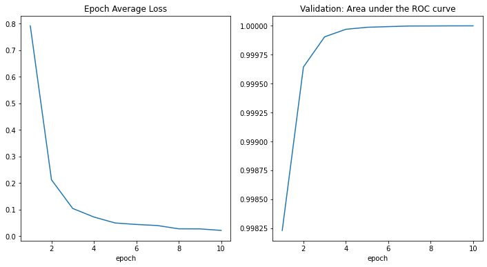
2. 総エポック数の設定、シャッフルとランダム変換を持ちますので、総てのエポックの訓練データは異なります。そしてこれは単なる get start チュートリアルですから、4 エポックだけ訓練しましょう。10 エポック訓練すれば、モデルはテストデータセットで 100% 精度を達成できます。
3. MONAI から DenseNet を使用して GPU デバイスに移します、この DenseNet は 2D と 3D 分類タスクの両方をサポートできます。
4. Adam optimizer を使用します。

device = torch.device("cuda:0")
model = DenseNet121(
    spatial_dims=2,
    in_channels=1,
    out_channels=num_class
).to(device)
loss_function = torch.nn.CrossEntropyLoss()
optimizer = torch.optim.Adam(model.parameters(), 1e-5)
epoch_num = 4
val_interval = 1

 

モデル訓練

エポックループとステップループを実行する典型的な PyTorch 訓練を実行し、そしてエポック毎後に検証を行ないます。ベストな検証精度を得た場合にはモデル重みをファイルにセーブします。

best_metric = -1
best_metric_epoch = -1
epoch_loss_values = list()
auc_metric = ROCAUCMetric()
metric_values = list()
for epoch in range(epoch_num):
    print('-' * 10)
    print(f"epoch {epoch + 1}/{epoch_num}")
    model.train()
    epoch_loss = 0
    step = 0
    for batch_data in train_loader:
        step += 1
        inputs, labels = batch_data[0].to(device), batch_data[1].to(device)
        optimizer.zero_grad()
        outputs = model(inputs)
        loss = loss_function(outputs, labels)
        loss.backward()
        optimizer.step()
        epoch_loss += loss.item()
        print(f"{step}/{len(train_ds) // train_loader.batch_size}, train_loss: {loss.item():.4f}")
        epoch_len = len(train_ds) // train_loader.batch_size
    epoch_loss /= step
    epoch_loss_values.append(epoch_loss)
    print(f"epoch {epoch + 1} average loss: {epoch_loss:.4f}")

    if (epoch + 1) % val_interval == 0:
        model.eval()
        with torch.no_grad():
            y_pred = torch.tensor([], dtype=torch.float32, device=device)
            y = torch.tensor([], dtype=torch.long, device=device)
            for val_data in val_loader:
                val_images, val_labels = val_data[0].to(device), val_data[1].to(device)
                y_pred = torch.cat([y_pred, model(val_images)], dim=0)
                y = torch.cat([y, val_labels], dim=0)
            y_onehot = [to_onehot(i) for i in y]
            y_pred_act = [act(i) for i in y_pred]
            auc_metric(y_pred_act, y_onehot)
            auc_result = auc_metric.aggregate()
            auc_metric.reset()
            del y_pred_act, y_onehot
            metric_values.append(auc_result)
            acc_value = torch.eq(y_pred.argmax(dim=1), y)
            acc_metric = acc_value.sum().item() / len(acc_value)
            if acc_metric > best_metric:
                best_metric = acc_metric
                best_metric_epoch = epoch + 1
                torch.save(model.state_dict(), 'best_metric_model.pth')
                print('saved new best metric model')
            print(f"current epoch: {epoch + 1} current AUC: {auc_result:.4f}"
                  f" current accuracy: {acc_metric:.4f} best AUC: {best_metric:.4f}"
                  f" at epoch: {best_metric_epoch}")
print(f"train completed, best_metric: {best_metric:.4f} at epoch: {best_metric_epoch}")

----------
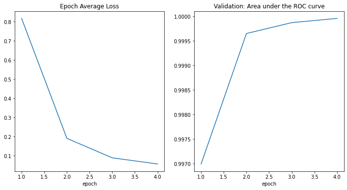
epoch 1/4
(...)
epoch 1 average loss: 0.8166
saved new best metric model
current epoch: 1 current AUC: 0.9970 current accuracy: 0.9582 best AUC: 0.9582 at epoch: 1
----------
epoch 2/4
(...)
epoch 2 average loss: 0.1908
saved new best metric model
current epoch: 2 current AUC: 0.9996 current accuracy: 0.9801 best AUC: 0.9801 at epoch: 2
----------
epoch 3/4
(...)
epoch 3 average loss: 0.0894
saved new best metric model
current epoch: 3 current AUC: 0.9999 current accuracy: 0.9899 best AUC: 0.9899 at epoch: 3
----------
epoch 4/4
(...)
epoch 4 average loss: 0.0573
saved new best metric model
current epoch: 4 current AUC: 1.0000 current accuracy: 0.9948 best AUC: 0.9948 at epoch: 4
train completed, best_metric: 0.9948 at epoch: 4

epoch 10 average loss: 0.0214
saved new best metric model
current epoch: 10 current AUC: 1.0000 current accuracy: 0.9993 best AUC: 0.9993 at epoch: 10
train completed, best_metric: 0.9993 at epoch: 10
CPU times: user 5min 2s, sys: 10.1 s, total: 5min 12s
Wall time: 9min 45s

 

損失とメトリックのプロット

plt.figure('train', (12, 6))
plt.subplot(1, 2, 1)
plt.title("Epoch Average Loss")
x = [i + 1 for i in range(len(epoch_loss_values))]
y = epoch_loss_values
plt.xlabel('epoch')
plt.plot(x, y)
plt.subplot(1, 2, 2)
plt.title("Validation: Area under the ROC curve")
x = [val_interval * (i + 1) for i in range(len(metric_values))]
y = metric_values
plt.xlabel('epoch')
plt.plot(x, y)
plt.show()

 

テストデータセットでモデルを評価する

訓練と検証の後、検証テスト上のベストモデルを既に得ています。モデルが堅牢であることと過剰適合していないことを確認するためにテストデータセット上で評価する必要があります。分類レポートを生成するためにこれらの予測を使用します。

model.load_state_dict(torch.load('best_metric_model.pth'))
model.eval()
y_true = list()
y_pred = list()
with torch.no_grad():
    for test_data in test_loader:
        test_images, test_labels = test_data[0].to(device), test_data[1].to(device)
        pred = model(test_images).argmax(dim=1)
        for i in range(len(pred)):
            y_true.append(test_labels[i].item())
            y_pred.append(pred[i].item())

from sklearn.metrics import classification_report
print(classification_report(y_true, y_pred, target_names=class_names, digits=4))

              precision    recall  f1-score   support

   AbdomenCT     0.9885    0.9916    0.9900       950
   BreastMRI     0.9967    0.9913    0.9940       918
         CXR     0.9980    0.9950    0.9965      1008
     ChestCT     0.9959    1.0000    0.9980       978
        Hand     0.9961    0.9961    0.9961      1036
      HeadCT     0.9947    0.9958    0.9953       950

    accuracy                         0.9950      5840
   macro avg     0.9950    0.9950    0.9950      5840
weighted avg     0.9950    0.9950    0.9950      5840

以上